Quickstart Guide
Get up and running with Pulseq on Philips in three simple steps.
Prerequisites
Before you begin, ensure you have:


- New to Pulseq? Check out the Pulseq Tutorials
- New to Philips? There are courses provided by Philips and Gyrotools

No MATLAB or Python?
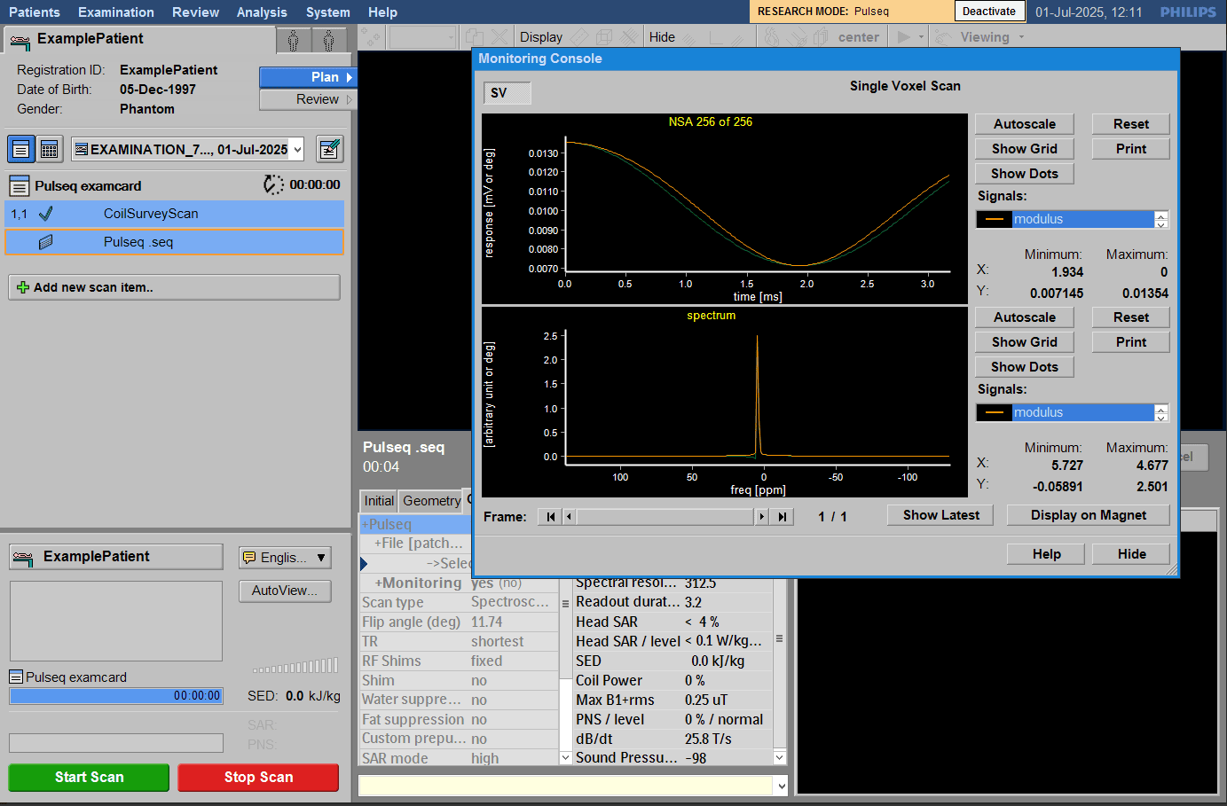
You can still follow along by downloading the example .seq files directly, or by using an online environment:![]()
Step 1: Get a Sequence File
You can either download a pre-made sequence file or create your own:

Start with one of our validated examples.
View Examples
Use PyPulseq or MATLAB to design a sequence.
Pulseq Tutorials
Minimal Example
Here's a simple Gradient Echo (GRE) sequence to get you started.
import math

import numpy as np

import pypulseq as pp


def main(plot: bool = False, write_seq: bool = False, seq_filename: str = 'gre_pypulseq.seq'):
    # ======
    # SETUP
    # ======
    # Create a new sequence object
    fov = 256e-3  # Define FOV and resolution
    Nx = 64
    Ny = 64
    alpha = 10  # flip angle
    slice_thickness = 3e-3  # slice
    TR = 12e-3  # Repetition time
    TE = 5e-3  # Echo time

    rf_spoiling_inc = 117  # RF spoiling increment

    system = pp.Opts(
        max_grad=28,
        grad_unit='mT/m',
        max_slew=150,
        slew_unit='T/m/s',
        rf_ringdown_time=20e-6,
        rf_dead_time=100e-6,
        adc_dead_time=10e-6,
    )

    seq = pp.Sequence(system)

    # ======
    # CREATE EVENTS
    # ======
    rf, gz, _ = pp.make_sinc_pulse(
        flip_angle=alpha * math.pi / 180,
        duration=3e-3,
        slice_thickness=slice_thickness,
        apodization=0.42,
        time_bw_product=4,
        system=system,
        return_gz=True,
        delay=system.rf_dead_time,
    )
    # Define other gradients and ADC events
    delta_k = 1 / fov
    gx = pp.make_trapezoid(channel='x', flat_area=Nx * delta_k, flat_time=3.2e-3, system=system)
    adc = pp.make_adc(num_samples=Nx, duration=gx.flat_time, delay=gx.rise_time, system=system)
    gx_pre = pp.make_trapezoid(channel='x', area=-gx.area / 2, duration=1e-3, system=system)
    gz_reph = pp.make_trapezoid(channel='z', area=-gz.area / 2, duration=1e-3, system=system)
    phase_areas = (np.arange(Ny) - Ny / 2) * delta_k

    # gradient spoiling
    gx_spoil = pp.make_trapezoid(channel='x', area=2 * Nx * delta_k, system=system)
    gz_spoil = pp.make_trapezoid(channel='z', area=4 / slice_thickness, system=system)

    # Calculate timing
    delay_TE = (
        math.ceil(
            (
                TE
                - (pp.calc_duration(gz, rf) - pp.calc_rf_center(rf)[0] - rf.delay)
                - pp.calc_duration(gx_pre)
                - pp.calc_duration(gx) / 2
                - pp.eps
            )
            / seq.grad_raster_time
        )
        * seq.grad_raster_time
    )
    delay_TR = (
        np.ceil(
            (TR - pp.calc_duration(gz, rf) - pp.calc_duration(gx_pre) - pp.calc_duration(gx) - delay_TE)
            / seq.grad_raster_time
        )
        * seq.grad_raster_time
    )

    assert np.all(delay_TE >= 0)
    assert np.all(delay_TR >= pp.calc_duration(gx_spoil, gz_spoil))

    rf_phase = 0
    rf_inc = 0

    # ======
    # CONSTRUCT SEQUENCE
    # ======
    # Loop over phase encodes and define sequence blocks
    for i in range(Ny):
        rf.phase_offset = rf_phase / 180 * np.pi
        adc.phase_offset = rf_phase / 180 * np.pi
        rf_inc = divmod(rf_inc + rf_spoiling_inc, 360.0)[1]
        rf_phase = divmod(rf_phase + rf_inc, 360.0)[1]

        seq.add_block(rf, gz)
        gy_pre = pp.make_trapezoid(
            channel='y',
            area=phase_areas[i],
            duration=pp.calc_duration(gx_pre),
            system=system,
        )
        seq.add_block(gx_pre, gy_pre, gz_reph)
        seq.add_block(pp.make_delay(delay_TE))
        seq.add_block(gx, adc)
        gy_pre.amplitude = -gy_pre.amplitude
        seq.add_block(pp.make_delay(delay_TR), gx_spoil, gy_pre, gz_spoil)

    # Check whether the timing of the sequence is correct
    ok, error_report = seq.check_timing()
    if ok:
        print('Timing check passed successfully')
    else:
        print('Timing check failed. Error listing follows:')
        [print(e) for e in error_report]

    # ======
    # VISUALIZATION
    # ======
    if plot:
        seq.plot()

    seq.calculate_kspace()

    # Very optional slow step, but useful for testing during development e.g. for the real TE, TR or for staying within
    # slew-rate limits
    rep = seq.test_report()
    print(rep)

    # =========
    # WRITE .SEQ
    # =========
    if write_seq:
        # Prepare the sequence output for the scanner
        seq.set_definition(key='FOV', value=[fov, fov, slice_thickness])
        seq.set_definition(key='Name', value='gre')

        seq.write(seq_filename)

    return seq


if __name__ == '__main__':
    main(plot=False, write_seq=True)
% set system limits
sys = mr.opts('MaxGrad', 22, 'GradUnit', 'mT/m', ...
    'MaxSlew', 120, 'SlewUnit', 'T/m/s', ...
    'rfRingdownTime', 20e-6, 'rfDeadTime', 100e-6, 'adcDeadTime', 10e-6);

seq=mr.Sequence(sys);           % Create a new sequence object
fov=256e-3; Nx=128; Ny=Nx;      % Define FOV and resolution
alpha=10;                       % flip angle
sliceThickness=3e-3;            % slice
TR=12e-3;                       % repetition time TR
TE=5e-3;                        % echo time TE
%TE=[7.38 9.84]*1e-3;            % alternatively give a vector here to have multiple TEs (e.g. for field mapping)

% more in-depth parameters
rfSpoilingInc=117;              % RF spoiling increment
roDuration=3.2e-3;              % ADC duration

% Create fat-sat pulse
% (in Siemens interpreter from January 2019 duration is limited to 8.192 ms, and although product EPI uses 10.24 ms, 8 ms seems to be sufficient)
% B0=2.89; % 1.5 2.89 3.0
% sat_ppm=-3.45;
% sat_freq=sat_ppm*1e-6*B0*lims.gamma;
% rf_fs = mr.makeGaussPulse(110*pi/180,'system',lims,'Duration',8e-3,...
%     'bandwidth',abs(sat_freq),'freqOffset',sat_freq);
% gz_fs = mr.makeTrapezoid('z',sys,'delay',mr.calcDuration(rf_fs),'Area',1/1e-4); % spoil up to 0.1mm

% Create alpha-degree slice selection pulse and gradient
[rf, gz] = mr.makeSincPulse(alpha*pi/180,sys,'Duration',3e-3,...
    'SliceThickness',sliceThickness,'apodization',0.42,'timeBwProduct',4,...
    'use','excitation');

% Define other gradients and ADC events
deltak=1/fov;
gx = mr.makeTrapezoid('x',sys,'FlatArea',Nx*deltak,'FlatTime',roDuration);
adc = mr.makeAdc(Nx,sys,'Duration',gx.flatTime,'Delay',gx.riseTime);
gxPre = mr.makeTrapezoid('x',sys,'Area',-gx.area/2,'Duration',1e-3);
gzReph = mr.makeTrapezoid('z',sys,'Area',-gz.area/2,'Duration',1e-3);
phaseAreas = ((0:Ny-1)-Ny/2)*deltak;
gyPre = mr.makeTrapezoid('y',sys,'Area',max(abs(phaseAreas)),'Duration',mr.calcDuration(gxPre));
peScales=phaseAreas/gyPre.area;


% gradient spoiling
gxSpoil=mr.makeTrapezoid('x',sys,'Area',2*Nx*deltak);
gzSpoil=mr.makeTrapezoid('z',sys,'Area',4/sliceThickness);

% Calculate timing
delayTE=ceil((TE - mr.calcDuration(gxPre) - gz.fallTime - gz.flatTime/2 ...
    - mr.calcDuration(gx)/2)/seq.gradRasterTime)*seq.gradRasterTime;
delayTR=ceil((TR - mr.calcDuration(gz) - mr.calcDuration(gxPre) ...
    - mr.calcDuration(gx) - delayTE)/seq.gradRasterTime)*seq.gradRasterTime;
assert(all(delayTE>=0));
assert(all(delayTR>=mr.calcDuration(gxSpoil,gzSpoil)));

rf_phase=0;
rf_inc=0;

% Loop over phase encodes and define sequence blocks
for i=1:Ny
    for c=1:length(TE)
        %seq.addBlock(rf_fs,gz_fs); % fat-sat
        rf.phaseOffset=rf_phase/180*pi;
        adc.phaseOffset=rf_phase/180*pi;
        rf_inc=mod(rf_inc+rfSpoilingInc, 360.0);
        rf_phase=mod(rf_phase+rf_inc, 360.0);
        %
        seq.addBlock(rf,gz);
        seq.addBlock(gxPre,mr.scaleGrad(gyPre,peScales(i)),gzReph);
        seq.addBlock(mr.makeDelay(delayTE(c)));
        seq.addBlock(gx,adc);
        %gyPre.amplitude=-gyPre.amplitude;
        seq.addBlock(mr.makeDelay(delayTR(c)),gxSpoil,mr.scaleGrad(gyPre,-peScales(i)),gzSpoil)
    end
end

%% check whether the timing of the sequence is correct
[ok, error_report]=seq.checkTiming;

if (ok)
    fprintf('Timing check passed successfully\n');
else
    fprintf('Timing check failed! Error listing follows:\n');
    fprintf([error_report{:}]);
    fprintf('\n');
end

%% prepare sequence export
seq.setDefinition('FOV', [fov fov sliceThickness]);
seq.setDefinition('Name', 'gre');

seq.write('gre.seq')       % Write to pulseq file
Step 2: Install the Interpreter
The interpreter is a Philips patch that you need to build and install.
The details on this process are available in the private GitHub repository
Research patches
The Pulseq interpreter is a patch, like any other. Patches can be wonderful, and might bring great features to your scanner.
However this patch, like others, is not made by Philips. You need to build the patch yourself, and you are responsible for its validation and usage.
Build and Install overview
- Get the code by adding the private GitHub repository as a new remote
- Checkout the interpreter branch if it is available for your scanner's relase
- If needed merge the code, into your own custom patch or branch
- Compile the code into a patch
- Test the patch and your
.seqfiles in the simulator - All okay? Copy over and enjoy the interpreter on your scanner!

More detailed instructions are available in the repository's README.
Follow all steps, including testing!
The above steps are a high-level overview. We strongly recommend following all steps in the provided README file.
If you're an experienced researcher, you might be tempted to skip some steps. Don't!
Every step is not only designed to take all safety precautions into account - they are also advised to simply provide you with the best experience.
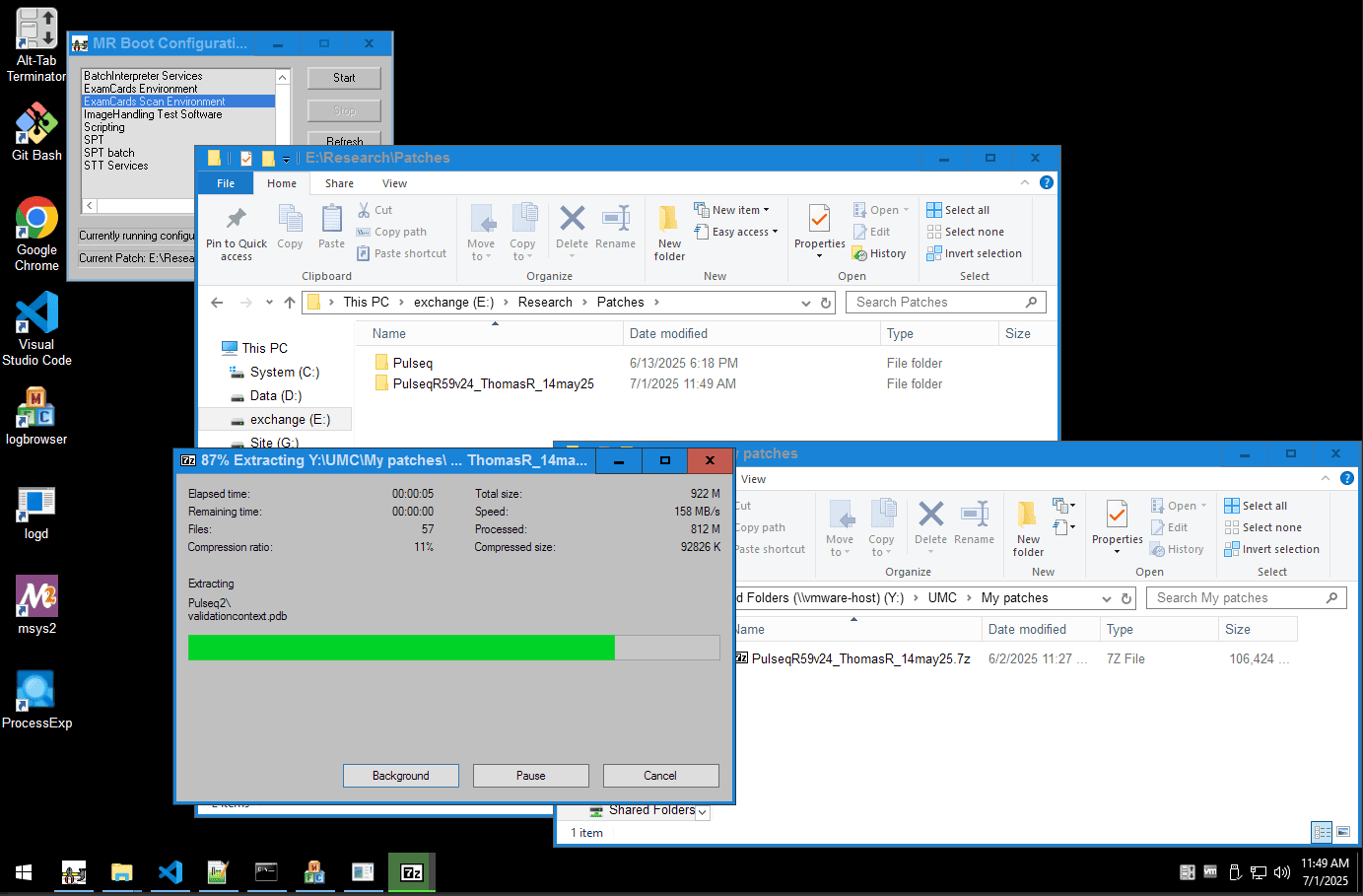
Step 3: Run Your Sequence
Copy over (and uncompress if needed) the patch folder, to the scanner's patch directory
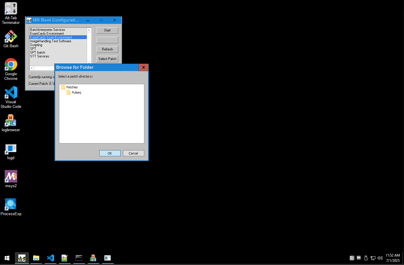
Activate the patch, for example, using the MR Boot Configuration window
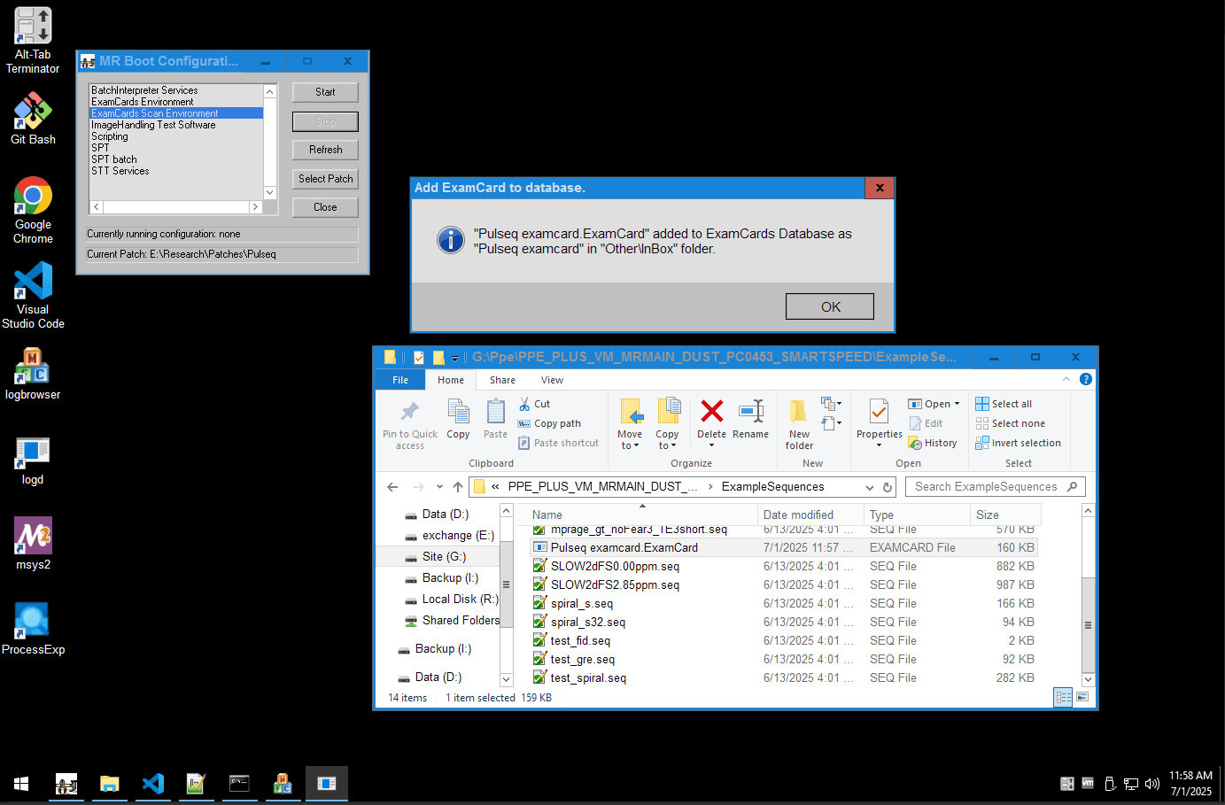
Double click on the .ExamCard file provided with the patch source code, to load it into the scanner's database
Open the "Pulseq .seq" scan, and select the sequence file (in the patch directory) to run
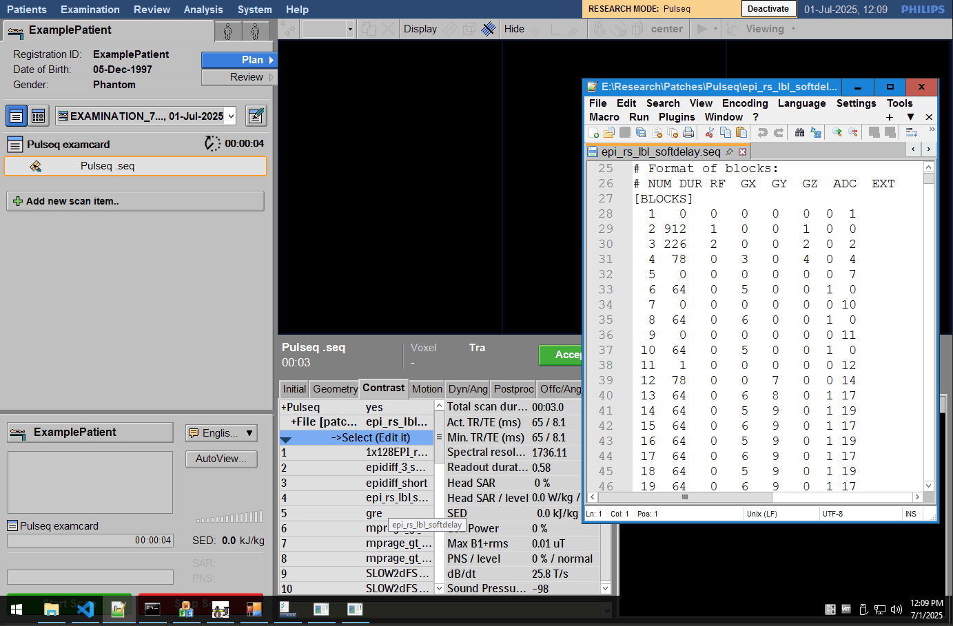
Hit "Start Scan" to run your sequence!
Next Steps
Now that you're set up, explore what else is possible:

Discover hybrid mode, pTx support, and more.
See Features
Browse complex sequences like EPI and Spiral.
View ExamplesGet help, contribute, and connect with other users.
Get in touch
How to Cite
If you use our Pulseq Interpreter in your research, please cite our work:
BibTeX Citation
@article{Roos2025,
  title = {pTx-Pulseq in hybrid sequences: Accessible \& advanced hybrid open-source MRI sequences on Philips scanners},
  author = {Thomas H. M. Roos and Edwin Versteeg and Mark Gosselink and Hans Hoogduin and
            Kyung Min Nam and Nicolas Boulant and Vincent Gras and Franck Mauconduit and
            Dennis W. J. Klomp and Jeroen C. W. Siero and Jannie P. Wijnen},
  journal = {Magnetic Resonance in Medicine},
  year = {2025},
  pages = {1--17},
  doi = {10.1002/mrm.30601}
}
APA Style
Roos, T., Versteeg, E., Gosselink, M., Hoogduin, H., Nam, K., Boulant, N., Gras, V., Mauconduit, F., Klomp, D., Siero, J. C. W., & Wijnen, J. (2025).
pTx-Pulseq in hybrid sequences: Accessible & advanced hybrid open-source MRI sequences on Philips scanners.
Magnetic Resonance in Medicine, 1, 1–17.
doi.org/10.1002/mrm.30601